The Theory of Causal Fermion Systems
Motivation in Examples
Motivation in Examples
Knowing that examples are very helpful for a first understanding, on this page we motivate in simple examples how the basic objects of the theory come about and how to think about them. In order to provide different perspectives, we give two different examples:
- Encoding spacetime structures in wave functions: Here the motivating question is how spacetime structures can be encoded in quantum mechanical wave functions.
- Formulating equations in discrete spacetimes: Here we begin with the example of a two-dimensional lattice system and ask the question how one can formulate physical equations in this discrete spacetime without making use of specific lattice structures like the nearest neighbor relations and the lattice spacing
- Toward the general definition of a causal fermion system: Here we explain how to get from the setting of the two examples to the general definition of a causal fermion system.
Encoding Spacetime Structures in Wave Functions
We begin with a quantum particle described by a quantum mechanical wave function $\psi$ satisfying the Klein-Gordon equation $(-\Box – m^2)\: \psi = 0$ in Minkowski space or in curved spacetime. Suppose that we have only access to the information contained in the absolute square $|\psi(x)|^2$ of this wave function. We ask the question: Given this information, what can we infer about the structure of spacetime? First, let the wave function $\psi$ be a solution evolved from compactly supported initial data. Then finite speed of propagation guarantees that the absolute square $|\psi(x)|^2$ vanishes outside the causal future of the support of the initial data. as is illustrated in the following figure:
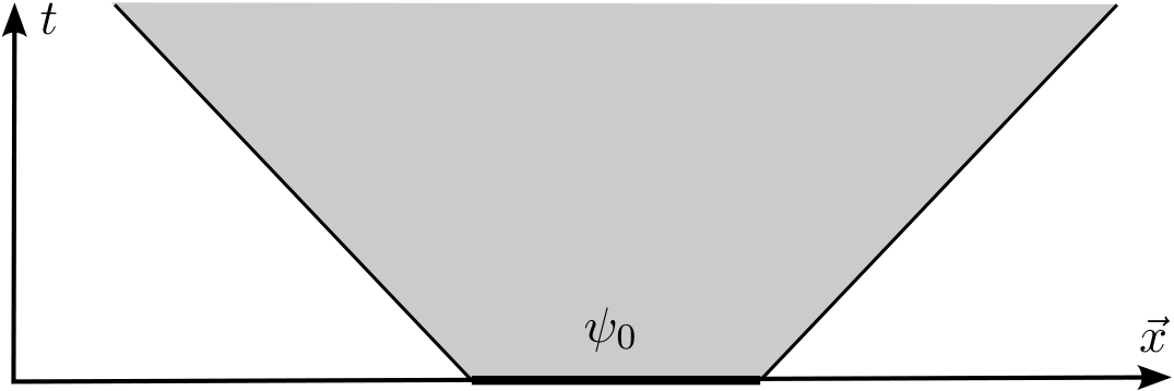
Therefore, the support of $|\psi(x)|^2$ contains some information about the causal structure of our spacetime. But, of course, there is only a limited amount of information which one can extract from a single wave function. However, if instead we probe classical spacetime with many wave functions, then we gain more information, as illustrated in the next figure:

If we aggregate the information contained in all wave functions evolved from compactly supported initial data, then we can extract the complete causal structure of our spacetime. We remark that this determines the metric up to a conformal factor [hkm, m77].
We next consider the situation if an electromagnetic field is present. Then the coupling of the scalar field to the electromagnetic field is described by the Klein-Gordon equation with minimal coupling $-(\partial_k – i e A_k) (\partial^k – i e A^k)\:\psi = m^2 \psi$. Now the wave functions are deflected by the electromagnetic force. Therefore, their absolute square also encodes information on the electromagnetic field. In order to retrieve this information, one can use the following procedure. Suppose that we have access to two wave function $\psi$ and $\phi$ and that we can also measure the absolute value of superpositions, i.e.
$\big| \alpha \psi(x) + \beta \phi(x) \big|^2 = \big| \alpha \psi(x) \big|^2 + 2 \text{Re} \big( \alpha \overline{\beta}\: \psi(x) \overline{\phi(x)} \big) + \big| \beta \phi(x) \big|^2 $
for arbitrary complex coefficients $\alpha$ and $\beta$. By varying these parameters, we can determine the quantity
$\overline{\psi(x)} \phi(x) \:,$
telling us about the correlation of the two wave function $\psi$ and $\phi$ at the spacetime point $x$. This allows us to probe the electromagnetic field as shown in the next figure:

Here we do not need to be specific on what “probing” exactly means (for example, one could determine deflection angles, recover the Aharanov-Bohm phase shifts of the wave function, etc.). All that counts is that we can get information also on the electromagnetic field. Generally speaking, the more wave functions we have to our disposal, the more information on the electromagnetic field can be obtained. It seems sensible to expect that, after suitably increasing the number of wave functions, we can recover both the spacetime structures and the matter fields therein from the knowledge of the absolute square of all these wave functions alone.
Now we go one step further and formulate the idea of encoding spacetime structures in a family of wave functions in mathematical terms. To this end, we consider a (for simplicity finite) number $f$ of linearly independent wave functions $\psi_1,\dots,\psi_f: \, \scrM \rightarrow \C$, mapping from a classical spacetime $\scrM$ into the complex numbers. On the complext vector space $\H$ spanned by these wave functions we introduce a scalar product $\la.|.\ra_\H$ by demanding that the wave functions $\psi_1,\ldots,\psi_f$ are orthonormal, i.e.
$\la \psi_k|\psi_l\ra_\H = \delta_{kl} \,.$
We thus obtain an $f$ dimensional Hilbert space $(\H, \la.|.\ra_\H)$. At any spacetime point $x \in \scrM$ we can now introduce the local correlation operator $F(x): \H \rightarrow \H$ at $x$ as the linear operator whose matrix representation in the basis $\psi_1,\ldots,\psi_f$ is given by
$\big(F(x)\big)^j_{\hphantom{j}k}=\overline{\psi_j(x)}\psi_k(x) \:.$
The diagonal entries of this matrix give the absolute squares of the wave functions, whereas the off-diagonal entries tell us about the correlation of the wave functions at the spacetime point $x$. Therefore, we refer to $F(x)$ as the local correlation operator. Alternatively, the local correlation operator is characterized in a basis-invariant form by the identity
$\la \psi|F(x)\phi\ra_\H=\overline{\psi(x)}\phi(x), \qquad \text{for all $\psi, \phi \in \H$} \:.$
By construction, the operator $F(x)$ is positive semi-definite and has rank at most one. We have thus constructed a map $F: \scrM \to \F$ from our classical spacetime $\scrM$ to the set $\F$ of positive semi-definite linear operators and of rank at most one on a Hilbert space of dimension $f$.
$\F:= \{ y \in \Lin(\H) \,|\, y \text{ positive semi-definite of rank at most one}\}$
This map encodes all the physical information contained in the wave functions of $\H$. As mentioned before, however, this information does not include the volume measure. Therefore, we introduce the volume measure as an additional structure. We can define a volume measure on the set $\F$ by the push-forward measure defined by
$\rho (\Omega):= \mu \big( F^{-1}(\Omega) \big) = \int_{F^{-1}(\Omega)} d\mu \:,$
where $\mu$ is the volume measure on $\scrM$ (i.e. $d\mu = d^4x$ in Minkowski space and $d\mu = \sqrt{|\det g|}\: d^4x$ in curved spacetime). We now have all the ingredients at hand needed to define a causal fermion system. The only modification is that, instead of complex wave functions, we will work with sections of a spinor bundle. One consequence of that is that the local correlation operator will no longer be positive semi-definite. They will still be of finite rank but instead with a fixed upper bound for the number of positive and negative eigenvalues. This leads to the basic definition of a causal fermion sytem.
Formulating Equations in Discrete Spacetimes
It is generally believed that for distances as small as the Planck scale, spacetime can no longer be described by Minkowski space or a Lorentzian manifold, but that it should have a different, possibly discrete structure. There exist different approaches to model such spacetimes, the simplest and most direct one perhaps being the replacement of Minkowski space by a discrete lattice, causal fermion systems being a different, more indirect approach. In any such approach one faces the challenge of how to formulate physical equations if one gives up the continuous structure of spacetime and thus can no longer use partial differential equations like the Klein-Gordon equation or the Dirac equation as physical equations.
To understand these challenges more vividly, we now consider the simple example of a spacetime lattice. For simplicity, we consider a two-dimensional lattice (one space and one time dimension), but higher-dimensional lattices could be described similarly. Thus let $\scrM \subset \R^{1,1}$ be a rectangular lattice in two-dimensional Minkowski space. We denote the spacing in time direction by $\Delta t$ and in spatial direction by $\Delta x$, as is shown in the following figure:
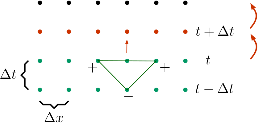
The usual procedure for setting up equations on a lattice is to replace derivatives by difference quotients, giving rise to an evolution equation which can be solved time step by time step according to deterministic rules.
As a concrete example, let us consider a discretization of the two-dimensional wave equation for a function $\phi: \scrM \to \C$ on the lattice,
\begin{align*}
0 = \Box \phi(t,x) &:= \frac{1}{(\Delta t)^2} \Big( \phi(t+\Delta t, x)
– 2 \phi(t, x) + \phi(t-\Delta t, x)\Big) \\
&\qquad – \frac{1}{(\Delta x)^2} \Big( \phi(t, x+\Delta x)
– 2 \phi(t, x) + \phi(t, x – \Delta x)\Big) \:.
\end{align*}
Solving this equation for $\phi(t+\Delta t, x)$ gives a rule for computing $\phi(t+\Delta t, x)$ from the values of $\phi$ at earlier times $t$ and $t-\Delta t$ (see again the above figure).
While this method for setting up equations on a discrete spacetime is indeed very simple and yields well-defined evolution equations, it also has several drawbacks:
- The above method of discretizing the continuum equations is very ad hoc. Why do we choose a regular lattice, why do we work with difference quotients? There are many other ways of discretizing the wave equation.
- The method is not background-free. In order to speak of the “lattice spacing,” the lattice must be thought of as being embedded in a two-dimensional ambient spacetime.
- The concept of a spacetime lattice is not invariant under general coordinate transformations. In other words, the assumption of a spacetime lattice is
not compatible with the equivalence principle.
In view of these shortcomings, the following basic question arises (we still remain in the setting of a spacetime lattice):
Can one find a way to formulate physical equations for fields on a spacetime lattice $\scrM$ without referring to concepts such as the nearest neighbor relation and the lattice spacing?
The answer to this question is yes, and we will now see how this can be done in the example of our two-dimensional lattice system. Although our example is somewhat oversimplified, this consideration will lead us quite naturally to the setting of causal fermion systems.
To describe our method for setting up equations, we pick up the contents of the previous section. To summarize, we consider $f$ linearly independent complex-valued wave functions $\psi_1, \ldots, \psi_f: \scrM \to \C$, now taken to be defined on the lattice $\scrM$.
A-priori, these wave functions are not assumed to satisfy any wave equation. On the complex vector space $\H$ spanned by these wave functions we introduce a scalar product $\la .|. \ra_\H$ by demanding that the wave functions $\psi_1, \ldots, \psi_f$ are orthonormal, i.e.
$\la \psi_k | \psi_l \ra_\H = \delta_{kl} \:.$
We thus obtain an $f$-dimensional Hilbert space $(\H, \la .|. \ra_\H)$. Note that the scalar product is given abstractly (meaning that it has no representation in terms of the wave functions as a sum over lattice points). Next, for any lattice point $(t,x) \in \scrM$ we introduce the so-called local correlation operator $F(t,x) : \H \rightarrow \H$ as the linear operator whose matrix representation in the basis $\psi_1,\ldots,\psi_f$ is given by
$(F(t,x))^j_k = \overline{\psi_j(t,x)} \psi_k(t,x) \:.$
The diagonal elements of this matrix are the absolute squares $|\psi_k(t,x)|^2$ of the corresponding wave functions. The off-diagonal elements, on the other hand, tell us about the correlation of the $j^\text{th}$ and $k^\text{th}$ wave function at the lattice point $(t,x)$. This is the reason for the name “local correlation operator.” This operator can also be characterized in a basis-invariant way by the relations
$\la \psi, F(t,x) \,\phi \ra_\H = \overline{\psi(t,x)} \phi(t,x) \:,$
to be satisfied for all $\psi, \phi \in \H$.
We now analyze some properties of the local correlation operators. Taking the complex conjugate of the above definition of the local correlation matrix, one sees immediately that this matrix is Hermitian. Stated equivalently independent of bases, the local correlation operator is a symmetric linear operator on $\H$. Moreover, a local correlation operator has rank at most one and is positive semi-definite. This can be seen by writing it as
$F(t,x) = e(t,x)^* e(t,x) \qquad \text{with} \qquad e(t,x) : \H \rightarrow \C\:,\quad \psi \mapsto \psi(t,x)$
and where $e(t,x)^*:\C \to \H$ is the adjoint of $e(t,x)$ as operator between the two Hilbert spaces $\H$ and $\C$.
It is useful to denote the set of all operators with the above properties by
\begin{align*}
\F := \big\{ & F \in \Lin(\H) \:\big|\: \text{$F$ is symmetric,} \\
& \text{positive semi-definite and has rank at most one} \big\} \:.
\end{align*}
Varying the lattice point, we obtain a mapping
$F : \scrM \rightarrow \F \:,\qquad (t,x) \mapsto F(t,x)$
shown in the next figure:
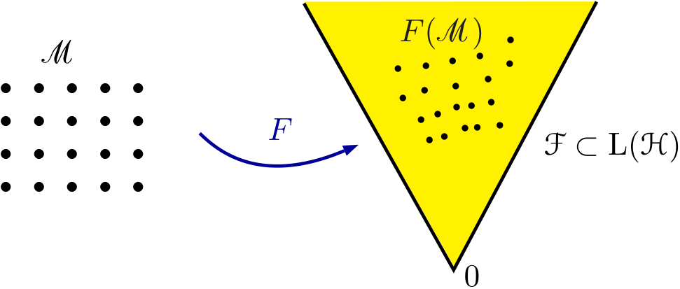
For clarity, we note that the set $\F$ is not a vector space, because a linear combination of operators in $\F$ in general has rank greater than one. But it is a conical set in the sense that a positive multiple of any operator in $\F$ is again in $\F$ (this is why in the above figure the set $\F$ is depicted as a cone).
We point out that the local correlation operators do not involve the lattice spacing or the nearest neighbor relation (as a matter of fact we never used that $\scrM$ is a lattive); instead they contain information only on the local correlations of the wave functions at each lattice point. With this in mind, our strategy for formulating equations which do not involve the specific structures of the lattice is to work exclusively with the local correlation operators, i.e. with the subset $F(\scrM) \subset \F$. In other words, in the aboe figure we want to disregard the lattice on the left and work only with the objects on the right.
How can one set up equations purely in terms of the local correlation operators? In order to explain the general procedure, we consider a finite number of operators $F_1, \ldots, F_L \in \F$. Each of these operators can be thought of as encoding information on the local correlations of the wave functions at a corresponding spacetime point. However, this “spacetime point” is no longer a lattice point, because the notions of lattice spacing and nearest lattice point have been dropped.
At this stage, spacetime is merely a point set, where each point is an operator on the Hilbert space. In order to obtain a “spacetime” in the usual sense (like Minkowski space, a Lorentzian manifold or a generalization thereof), one needs additional
structures and relations between the spacetime points. Such relations can be obtained by multiplying the operators. Indeed, the operator product $F_i \,F_j$ tells us about correlations of the wave functions at different spacetime points. Taking the trace of this operator product gives a real number. Our method for formulating physical equations is to use these properties of operators to set up a variational principle. This variational formulation has the advantage that symmetries give rise to conservation laws by Noether’s theorem (→ Nother-like theorems). Therefore, we want to minimize an action $\Sact$ defined in terms of the operators $F_1,\ldots,F_L$.
A simple example is to
$\text{minimize} \qquad \Sact(F_1, \ldots, F_L) := \sum_{i,j=1}^L \text{Tr} (F_i \,F_j)^2$
under variations of the points $F_1,\ldots, F_L \in \F$. In order to obtain a mathematically sensible variational principle, one needs to impose certain constraints. Here we do not enter the details, because the present example is a bit too simple. But it has a similar structure as the causal action principle and motivates the basic definition of a causal fermion system (→ Basic definitions).
A more physical example is to describe Minkowski space as a causal fermion system. Other simple examples are the causal variational principle on the sphere or the explicit examples in [intro, Chapter 20]. For the examples, one should keep in mind that a causal fermion system describes spacetime as well as all structures therein. Therefore, a too simple example cannot contain all the important physical structures.
Toward the General Definition of a Causal Fermion System
In order to get from the above examples to the general setting of causal fermion systems, we extend the above constructions in several steps:
- The previous example works similarly in higher dimensions,
in particular for a lattice $\scrM \subset \R^{1,3}$ in four-dimensional Minkowski space. This has no effect on the resulting structure of a finite number of distinguished operators $F_1, \ldots, F_L \in \F$. - Suppose that we consider multi-component wave functions $\psi: \scrM \to \C^N$. Then, clearly, we cannot directly multiply two such wave functions pointwise as was done above. However, assuming that we are given an inner product on $\C^N$, which we denote by $\Sl .|. \Sr$ (in mathematical terms, this inner product is a non-degenerate sesquilinear form; we always use the convention that the wave function in the first argument is complex conjugated), we can adapt the above definition of the local correlation operator to
\[ (F(t,x))^j_k = -\Sl \psi_j(t,x) | \psi_k(t,x) \Sr \]
(the minus sign merely is a useful convention). The resulting local correlation operator is no longer an operator of rank at most one, but it has rank at most $N$ (as can be seen for example by writing it in the form $F(t,x)=-e(t,x)^* e(t,x)$ with $e(t,x) : \H \rightarrow \C^N, \psi \mapsto \psi(t,x)$). If the inner product $\Sl .|. \Sr$ on $\C^N$ is positive definite, then the operator $F(t,x)$ is negative semi-definite. However, in the physical applications in mind, this inner product will {\em{not}} be positive definite. Indeed, a typical example in mind is that of four-component Dirac spinors. The Lorentz invariant inner product $\overline{\psi} \phi$ on Dirac spinors in Minkowski space (with the usual adjoint spinor $\overline{\psi} := \psi^\dagger \gamma^0$) is indefinite of signature $(2,2)$. In order to describe systems involving leptons and quarks, one must take direct sums of Dirac spinors, giving the signature $(n, n)$ with $n \in 2\N$. With this in mind, we assume more generally that
\[ \Sl .|. \Sr \quad \text{has signature $(n,n)$ with $n \in \N$}\:. \]
Then the resulting local correlation operators are symmetric operators of rank at most $2n$, which (counting multiplicities) have at most $n$ positive and at most $n$ negative eigenvalues. - Finally, it is useful to generalize the setting such as to allow for continuous spacetimes and for spacetimes which may have both continuous and discrete components. In preparation, we note that the sums over the operators $F_1,\ldots, F_L$ in the lattice example can be written as integrals,
\[ \Sact(\rho) = \int_\F d\rho(x) \int_\F d\rho(y)\: \text{Tr}(xy)^2 \:, \]
if the measure $\rho$ on $\F$ is chosen as the sum of Dirac measures supported at these operators,
\[ \rho = \sum_{i=1}^L \delta_{F_i} \:. \]
In this formulation, the measure plays a double role: First, it distinguishes the
points $F_1, \ldots, F_L$ as those points where the measure is non-zero, as is made mathematically precise by the notion of the support of the measure
\[ \text{supp}\, \rho = \{F_1, \ldots, F_L \}\:. \]
Second, a measure makes it possible to integrate over its support, an operation which in the above example reduces to the sum over $F_1, \ldots, F_L$.
Now one can extend the setting simply by considering the above action for more general measures on $\F$ (like for example regular Borel measures). The main advantage of working with measures is that we get into a mathematical framework in which such variational principles can be studied with powerful analytic methods.
Mathematical Introduction
Do you want to see the mathematical details?

Claudio Paganini
Author