The Theory of Causal Fermion Systems
Minkowski Space as a Causal Fermion System
Prerequisites
Continue Reading
Related Topics
Minkowski Space as a Causal Fermion System
Here it is described how Minkowski space can be described by a causal fermion system. Apart from illustrating the structures of a causal fermion system, this example is also the starting point for the analysis of the causal action principle in Minkowski space. More details on this example can be found in [cfs16, Section 1.2] and [Op20].
Construction of a Causal Fermion System in Minkowski Space
We first give the basic construction and explain it afterward. Let $\scrM$ be four-dimensional Minkowski space. We consider the Dirac equation
\[ i \gamma^j \partial_j \psi = m \psi \:. \]
On the smooth and spatially compact solutions of the Dirac equation we consider the usual scalar product
\[ (\psi | \phi)_m = \int_{\R^3} \overline{\psi(t, \vec{x} )} \gamma^0 \phi(t, \vec{x} )\: d^3x \]
where $\overline{\psi}=\psi^\dagger \gamma^0$ is the adjoint spinor. This scalar product is time independent due to current conservation. Taking the completion gives the Hilbert space $(\H_m, (.|.)_m)$
We now choose $(\H, \la .|. \ra_\H)$ as the subspace of all negative-energy solutions of the Dirac equation. The construction of the causal fermion system involves an ultraviolet regularization. To this end, given a regularization length $\varepsilon>0$, one introduces a regularization operator $\mathfrak{R}_\varepsilon$ which maps to continuous wave functions,
\[ \mathfrak{R}_\varepsilon \::\: \H \rightarrow C^0(\scrM, \C^4) \:. \]
Next, for any spacetime point $x=(t, \vec{x})$, we introduce the local correlation operator $F^\varepsilon(x)$ as the unique linear operator on $\H$ which satisfies the relation
$\la \psi | F^\varepsilon(x) \phi \ra_\H = -\overline{(\mathfrak{R}_\varepsilon \psi)(x)} (\mathfrak{R}_\varepsilon \phi)(x)$ for all $\psi, \phi \in \H$
The local correlation operator $F^\varepsilon(x)$ encodes information on the local densities and correlations of all the wave functions in $\H$ at the spacetime point $x$. By construction, the operator $F^\varepsilon(x)$ has finite rank, is symmetric and (counting multiplicities) has at most two positive and two negative eigenvalues. Thus it is an operator of $\F$ if we choose the spin dimension two.
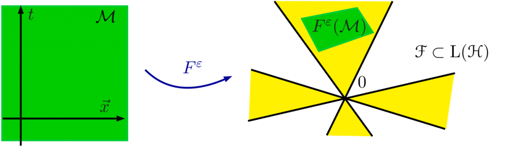
Varying the spacetime point $x$, we obtain the local correlation map $F : \scrM \rightarrow \F$:
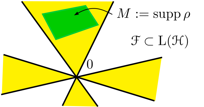
Finally, we introduce the measure $\rho$ as the push-forward of the volume measure $d\mu := d^4x$ under this mapping,
\[ \rho := (F^\varepsilon)_* \mu \]
(i.e. $\rho(\Omega) := \mu((F^\varepsilon)^{-1}(\Omega))$). We thus obtain a causal fermion system $(\F, \H, \rho)$ of spin dimension two.
Interpretation of the Construction
As the above construction is of central importance for the understanding of causal fermion systems, it requires a detailed explanation. Before beginning, we point out that the causal fermion system only contains partial information on the system. Indeed, the structures of Minkowski space (like geometry, causality) get lost. Thus the causal fermion system describes only the right side of the above picture:
This raises the immediate question whether these structures are still encoded in the causal fermion system. The answer is yes, because it turns out that the inherent structures of the causal fermion system (causal structure, spin spaces and wave functions as well as the geometric structures) give back the corresponding structures of Minkowski space in the limit $\varepsilon \searrow 0$ when the regularization is removed (for details see [cfs16, Section 1.2]). For example, the kernel of the fermionic projector goes over to the two-point distribution
\[ P(x,y) = \int \frac{d^4k}{(2 \pi)^4}\: \big(k^j \gamma_j + m)\: \delta(k^2-m^2)\: e^{-i k (y-x)} \:, \]
which is composed of all the negative-energy solutions of the Dirac equation.
The choice of $\H$ as all the negative-energy solutions of the Dirac equation realizes Dirac’s original concept that in the vacuum, all the states of negative energy should be occupied (Dirac sea). In the theory of causal fermion systems, this concept is taken seriously. However, the original problems of this concept (like the infinite negative energy density of the sea) do not occur because the Dirac sea drops out of the Euler-Lagrange equations corresponding to the causal action principle.
The regularization operator can be thought of as “smoothing” the wave functions on a microscopic scale. As a simple example, the regularization operator can be chosen as a convolution with a smooth test function. The length scale $\varepsilon$ can be thought of as the Planck length. In the theory of causal fermion systems, the regularization is not merely a technical tool in order to make divergent expressions finite, but it realizes the concept that on microscopic length scales the structure of spacetime itself is modified. Thus we always consider the regularized objects as the physical objects.
Particles, Anti-Particles and Interacting Systems
In order to describe systems involving particles and/or anti-particles, following Dirac’s hole theory one extends $\H$ by Dirac solutions of positive energy and/or removes vectors of negative energy. Bosonic fields (like electromagnetic or gravitational fields), on the other hand, correspond to collective “excitations” of the Dirac sea and the particle wave functions. In order to make this picture mathematically precise, one makes use of the fact that in a suitable limit $\varepsilon \searrow 0$, the measure $\rho$ describing the Minkowski vacuum is a critical point of the causal action. If particles and/or anti-particles are present, this is no longer the case. In order for these measures to become again critical points, they must be perturbed, leading to an interaction of the particles which (again in the limit $\varepsilon \searrow 0$) can be described by bosonic fields. This procedure is carried out sytematically and in computational detail in the so-called continuum limit.
→ The continuum limit
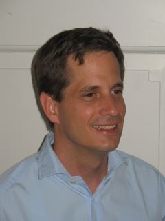
Felix Finster
Author