The Theory of Causal Fermion Systems
Osculating Vacua
Prerequisites
Continue Reading
Related Topics
Osculating vacua
The spacetime $\tilde{M}:= \text{supp} \tilde{\rho}$ describing an interacting system does not need to have a smooth manifold structure. Instead, it could have a non-smooth or even discrete structure. Nevertheless, in many situations it is useful to approximate spacetime locally by a vacuum spacetime $M:= \text{supp} \rho$. More precisely, one describes $\tilde{M}$ near a spacetime point $p \in \tilde{M}$ by a vacuum spacetime $M_p$ which is obtained from $M$ by a unitary transformation acting on the ambient space of operators $\F$. This concept is illustrated in the example of a discrete spacetime as follows:
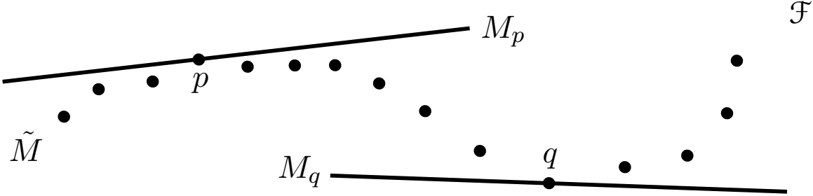
We refer to $M_p$ as the osculating vacuum at $p$. Osculations can be regarded as a generalization of the concept of the tangent space in differential geometry to the non-smooth setting. The osculating vacuum can be characterized by a corresponding variational principle.
The $\L$-Calculus
Having chosen an osculating vacuum at every spacetime point $p \in \tilde{M}$, one can adapt many concepts from differential topology to the non-smooth setting. In [FKT26] an exterior calculus for differential forms is developed (even in the more general setting of causal variational principles). One gets generalizations of the de Rham cohomology and glueing constructions. Moreover, Stokes’ theorem and the Gauß divergence theorem have natural generalizations to this setting.
The $\L$-Geometry
Under the additional assumption that $\tilde{M}$ has a smooth manifold structure, one can go one step further and use osculating vacua to also introduce structures familiar from differential geometry. The starting point is the observation that the osculation $M_p$ gives rise to a distinguished chart denoted by
$$ \phi_p : U \subset \tilde{M} \rightarrow M_p \:,\qquad \phi_p(\tilde{x}) :=
\frac{1}{\mathfrak{s}} \int_{M_p} \L(\tilde{x},y)\: y\: d\rho_p(y) \:, $$
Using these charts as analogs of Gaussian charts in Riemannian geometry, one gets a connection $\nabla^\L$ on the tangent bundle $T \tilde{M}$. This connection gives rise to a corresponding curvature tensor.
Moreover, one can define a Riemannian metric $g$ by
$$ g^{jk}(p) := \frac{1}{\mathfrak{s} \delta^2} \int_{M_p} \L(p,y)\: y^j y^k\: d\rho_p(y) $$
(here the proper normalization constant $\delta$ is the range of the Lagrangian; it can be identified with the Planck length).
A Lorentzian Metric
In order to get the connection to Lorentzian geometry, one introduces the regularizing vector field $u$ by
$$ u(p) := \frac{1}{\mathfrak{s}} \int_{M_p} \L(p,y)\: \mathscr{C}(p,y)\: y\: d\rho_p(y) \:, $$
where $\mathscr{C}$ is the time direction functional. The Lorentzian metric $\eta$ is introduced as the flip metric of the above Riemannian metric,
$$ \eta^{kl} = \frac{4}{3} \hat{u}^k \hat{u}^l – g^{kl} \:, $$
where $\hat{u}$ is the regularized vector field normalized with respect to $g$. This Lorentzian metric is compatible with the causal structure.
Ricci Curvature and the Einstein Equations
In general, the connection $\nabla^\L$ is not metric (neither with respect to $g$ nor with $\eta$). But the deviation is of higher oder in the range $\delta$ of the Lagrangian (to be identified with the Planck length). The key point is that the Ricci tensor of the $\nabla^\L$-connection has a divergence structure, making it possible to employ the Euler-Lagrange equations of the causal action principle. This gives rise to a derivation of the Lorentzian Einstein equations
$$ R^\eta_{il} -\frac{1}{2}\: R^\eta\, \eta_{il} = T_{il} \:, $$
where the energy-momentum tensor $T_{il}$ is of order $\mathcal{O}(\delta^2)$ and has an explicit expansion in powers of $\delta.

Felix Finster
Author