In the discussion of the continuum limit we briefly mentioned the difficulty of extracting information about the properties of our physical world from the Euler–Lagrange equation of the causal action principle (assuming for now that the framework of causal fermion systems provides an accurate model for our physical world). In what follows, we will make use of the fact that the regularized Dirac sea vacuum is a minimizer of the causal action in the continuum limit. Therefore, denoting the corresponding measure by $\rho_M$,
\[ \rho_M \in \mathcal{B}_{\mathcal{H}}(\mathcal{F}) \:, \]
where $\mathcal{B}_{\mathcal{H}}(\mathcal{F})$ is the set of all minimizing measures on $\F$ on a Hilbert space $\mathcal{H}$ (again choosing the spin dimension $n=2$).
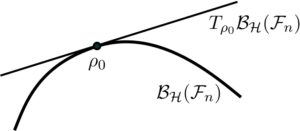
As a first step towards clarifying the meaning of the Euler-Lagrange equation is to consider linear perturbations of the measure $\rho_M$ which preserve the Euler-Lagrange equations. Mathematically, such linear perturbations satisfy the linearized field equations. Geometrically, they can be visualized as the tangent space to $\mathcal{B}_{\mathcal{H}}(\mathcal{F})$ at the minimizer $\rho_0 := \rho_M$. We will denote this tangent space by $T_{\rho_0}\mathcal{B}_{\mathcal{H}}(\mathcal{F})$. Thus this tangent space is formed of all measures $\rho_0+\lambda \delta \rho$ such that $\rho_0$ satisfies the Euler-Lagrange equations of the causal action principle, and $\delta \rho$ satisfies the linearized field equations.
When discussing the continuum limit, we already mentioned that in a causal fermion system, the Hilbert space is represented by wave functions in spacetime (the physical wave functions; see also the mathematics section → spin spaces and wave functions). The causal fermion system can be constructed from the physical wave functions by forming the local correlation operators. If we perturb the physical wave functions, we change the local correlation map $F$, which maps the spacetime manifold into $\F$ and thus defines the causal fermion system. In this way, we can relate a perturbation of the physical wave functions to a perturbation of the measure of the causal fermion system. Parametrizing the perturbation by $\lambda$, this procedure is summarized as follows,
\psi_i&\longrightarrow \psi_i^\lambda \qquad \text{with }\psi_i=\lim_{\lambda\rightarrow 0}\psi_i^\lambda\\
& \, \, \Downarrow\\
F(x)& \longrightarrow F^\lambda(x)\\
& \,\, \Downarrow\\
\rho_0(\Omega):= \mu(F^{-1}(\Omega))&\longrightarrow \rho_\lambda(\Omega):= \mu \big( (F^\lambda)^{-1}(\Omega) \big) \:,
\end{align}
where $\mu=d^4x$ is the four-dimensional volume measure in Minkowski space. Now we can linearize $\rho_\lambda$ in $\lambda$ around $\rho_0$ and verify whether the linearized modification lies in $T_{\rho_0}\mathcal{B}_{\mathcal{H}}(\mathcal{F})$, hence whether the linearized perturbation satisfies the linearized field equations. We only allow for those modifications of the configuration of the physical wave functions $\psi_i \longrightarrow \psi_i^\lambda $, with $\psi_i=\lim_{\lambda\rightarrow 0}\psi_i^\lambda$, which generate a modification of the measure $\rho_\lambda$ which obeys the linearized field equations.
The discussion presented here is but a sketch of the argument (for more details see the mathematics section → The continuum limit). In addition to the perturbation parameter $\lambda$, we will have the regularization parameter $\varepsilon$, and the linearized field equations need to be satisfied asymptotically as $\varepsilon \searrow 0$ in a suitable sense. Moreover, one must go beyond linear perturbation theory and treat the perturbations of the measure nonlinearly (for a systematic treatment see [perturb17]).
To give an example, we can modify the physical wave functions from the Dirac sea configuration by inserting an arbitrary four-vector potential into the Dirac equation,
(i \gamma^\mu\nabla_\mu -m) \psi_i(x)&=0\\
\downarrow \qquad & \\
(i \gamma^\mu\nabla_\mu + \lambda A^\mu -m) \psi_i^\lambda(x)&=0
\end{align}

Claudio Paganini
Author